Exercise #13: UAS Flights

Introduction

Earlier in the semester the class was able to learn the basics of Unmanned Aerial Systems (UAS) and experiment with operating these devices on a computer simulator. During this exercise we were able to learn and observe what the pre-flight protocols, mission planning, and actual flights consisted of. It is very, very important to be prepared and plan before going into the field to collect data. This exercise included flying two different UAS platforms: the IRIS (Fig 1) and a Matrix (Fig 2).

Figure 1. The IRIS platform flown during the exercise.

Figure 2. The Matrix platform flown during the exercise.

 

Study Area

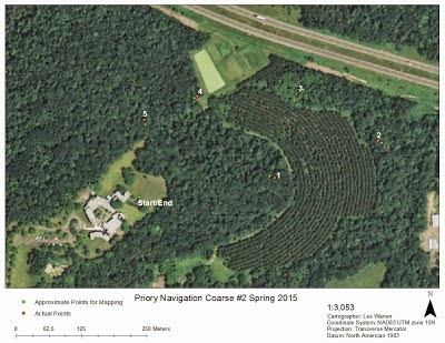
The study area for this exercise was once again the Priory (Fig 3). The Priory allowed wide-open spaces with a low volume of people or tall objects.

 

The weather consisted of:

        *Temperature: 52 degrees Fahrenheit

        *Cloud Cover: Cloudy, Stratus

        *Wind: 6-8mph S-SE; Gusty   

 

Figure 3. The UWEC Priory. This was the study area for the given exercise.

 

 



Mission Planning

 



One important aspect of flying UAS platforms is to create a Flight Mission. The Flight Mission communicates from the base station (either a computer (Fig. 4) or tablet (Fig. 5)) to the platform. Along with being connected to satellites and GPS, the base station controls the platforms movements if set on autopilot. This autopilot can be overridden at anytime by the Pilot. There are various base stations that can be used and each have their pros and cons. By using a computer, a person has more options and abilities to create more complex missions, but a computer is also very bulky and large. A tablet is light and easily to be carried, but has less options associated with it.

There are two ways in which a mission can be created. Either the manual plotting of points can be made over the given area or the computer can plot the points. By drawing a polygon shape over the AOI, the program will automatically (Fig 4). The specs of the senor or camera will depend on the number of points needed. The point mark areas the unit will turn or change direction.

Figure 4. The base station with the mission polygons drawn over the AOI.

 

 



Figure 5. Example of a tablet used when flying UAS units.

Pre-Flight 

One of the most important parts of flying a UAS platform is preforming a pre-flight checklist (Fig 6; Fig 8). By creating a checklist, like the one below, it ensures both a successful flight and that it is safely done. Safety of yourself and others is extremely important when flying a UAS platform. If something would not be fully connected, the unit could descend and cause injury, but also it could destroy the unit and sensor itself.

Safety is most definitely important, but so is a successful flight. If the sensor is not properly connected or the mission is not properly set up then it cause no data to be collected. This is a waste of time and money. By double checking oneself issues like this can be avoided.

Figure 6. Preforming the pre-flight checklist.

Pre-Flight Checklist (Fig 7)

1. Check Weather Conditions and Record

On Platform
2. Check Electrical Connections
3. Check Frame Connections
4. Check Motor Connections
5. Props Secure?
6. Props not cracked or chipped
7. Battery Secure?
8. Antenna Secure?
9. Sensor Connected?

Power Up Sequence
10. Green Light on Platform? (Indicates connected to Satellites/GPS)
11. Connect to Platform from Base Station
12. Batteries over 95%?
13. Transmitter on? Batteries charged?
14. Record number of available satellites
15. Mission Created?
16. Mission Secure? Area Clear?
17. Mission Sent?
18. Sensors on? At ready?

Take off Sequence
19. Throttle down?
20. Platform on
21. Spectators clear?
22. Kill switch off?
23. Clear for Launch
24. Activate Auto-pilot

Figure 8. Example of the pre-flight checklist on the base computer. It is important to recorded information like this to prevent failure and issues in the future.

 

 

 

Flights

 

Once the Flight Mission and Pre-Fight checklist have been completed, it is time to flight. By continuing with the checklist, the power-up and flight sequences can be followed (Fig 7). One of the most important concepts of flying is COMMUNICATION! The Pilot in Command and Unit Pilot must always be communicating. Once the unit is launched, variables like the number of satellites, if the platform is on coarse, and where is the platform located must always be watched. If something goes wrong, the Pilot in Command can abort the mission and the platform will automatically land itself (autopilot) or it can be manually landed. Just because the unit is on autopilot, it is extremely important to keep your eyes on it at all times incase an issue would occur.

 

Once a mission has been completed, it is important to fill out a Post Mission Log. By doing so, this is a place that issues and problems can be recorded to used for reference in the future. Things that would have gone into our log would have been the battery issues that included dead batteries, but also not to interchange batteries between controllers.

 

Pictures of the flights:

 

 

 

Data

 

Once the flight has been successfully flown, the data can be downloaded and processed through the software. With advancements in software, data can now be precessed right in the field. This has major advantages since a person can make sure the collection process was a success and all areas were covered. The software can process the image tiles into different photographs like RBG and IR.

 

Examples of the mosacis made in the field from the flight of the Matrix platform:

 

 

Final Remarks

 

This was an extremely educational and awesome experience. UAS units and technology are definitely the frontier of Geospatial Technology. I hope in the future that I will be able to learn more able this technology and utilize it in my research. 

 

Exercise #12: GPS Navigation

Introduction

Last week we were able to learn and utilize traditional navigation skills by navigating to pre-selected and placed points in the Priory. This week we were given the opportunity to build our own coarse for future classes. By creating a project onto a GPS unit (we chose the Trimble Juno Unit) we were then to navigate to points of our choice, mark the trees, and record the points.

Study Area

Once again this week we were at the UWEC Priory (Fig 1). Our study area was divided up into a different area for each given group. This was so the courses would not overlap or be located in one portion of the area. Our group had the far Northeast corner. The weather was Sunny, mid 70 degrees Fahrenheit, and little to no wind.

\

Figure 1. The UWEC Priory.

Methods

Once our group was given the selected area for our coarse, we took the paper maps we had created earlier in the semester and used last week and plotted points where we felt necessary. We wanted to make sure the points included distance, terrain, and were easily able to be navigated to within the class period. By having a project created on the Juno Unit (Fig 2), the Priory satellite imagery was available for us to use. This was our means to navigating to the points we selected. Once the points were navigated to, we were to mark the tree with the pink ribbon, label the ribbon with the group number and point number, and take a picture. The pictures of the five (5) points can be seen below (Fig 3-7).

Figure 2. The Trimble Juno 3D GPS unit used for the activity.

 

 

 

Figure 3. Point #2-1 for Coarse #2.

 

 

Figure 4. Point #2-2 for Coarse #2.

 

Figure 5. Point #2-3 for Coarse #2.

 

Figure 6. Point #2-4 for Coarse #2.

  

Figure 7. Point #2-5 for Coarse #2.

 

 

The points that we plotted were then loaded back into ArcMap and mapped (Fig 8). This also allowed us to create a Shapefile to submit so the data could be recorded for future classes. The attribute table gives the location of the points (in UTM) and also notes about the location of the tree.

 

 

Figure 8. Map of Coarse #2. The green dots represent the planned spot for the points, while the red dots are the actual locations of the points.

 

Figure 9. Attribute table of the points for Coarse #2.

 



 

Discussion

 

This exercise was extremely helpful with refreshing the skills we learned earlier in the semester, but also applying those skills to a navigation situation. Although you would think it would be easy to navigate to these points, there are still errors associated with the GPS unit. Looking at the map above, not one of the points match up exactly. This could be due to a low satellite frequency on the GPS or the group just saying we were "close enough" and marked the point. You still also need to account for terrain and obstacles while navigating.  

Exercise #11: Traditional Navigation

Introduction


Earlier in the semester, the class had created maps to be used later for a traditional navigation exercise. This week we completed that exercise. We were given printed versions of the maps we made, coordinates to travel to, and a compass to give bearing from point to point. This is a skill that is most defiantly needed since GPS technology is not always available depending on the area you are in and studying.





Study Area


The study area for this exercise was the University of Wisconsin- Eau Claire (UWEC) Priory (Fig 1). This is a very secluded area that is heavily wooded with trees and small brush. The weather included Sunny skies and mid 60 degree temperatures.

Figure 1. Aerial image of the UWEC Priory. This was the site for the traditional navigation.

Methods


The purpose of this exercise was to take a traditional map (Fig 2) and try to accurately plot given points and navigate from point to point and end back where we started. To do so, we first had to plot the points. The points were given to us in UTM coordinates. How accurate we were definitely depended on the scaling of our maps and grid scale.


Next, we were given our compasses and needed to calculate the azimuths from point to point. The first step is to set the compass on the map (not on or near any metal surfaces) and line it up with the first point and the point of interest (Fig 3). It is important to make sure the arrow of travel is going in the correct direction (pointed towards point of interest). Next, turn the bearing on the compass so that North is accurately pointing North (Fig 4). Reading the degrees at the arrow of travel and this is the azimuth to use while traveling to that point (Fig 5).


Do this for all point to point travels and record since it is much easier to do on a flat surface compared to out in the woods. You can calculate the distances by using the scale bar so that you an rough estimate of how far is needed to travel.


When traveling, keep the red arrow (north arrow) lined up with the red outline and keep traveling towards the arrow.

Figure 2. Map created in previous exercise of the Priory. The map with the UTM grid was used to complete the exercise.

 

 

Figure 3. First step in calculating the azimuth. Line the compass up with the start point and point of interest. It is import to make sure the arrow of travel is in the correct direction.

Figure 4. Second step in calculating azimuth. Turn the compass bearing so that North is accurately pointing North.

Figure 5. Step three of calculating the azimuth. Read the degrees at the arrow of travel.

Figure 6. Set the azimuth and keep "Red in the Shed" (line red arrow up with red outline) and travel to desired point.

 

Discussion


This is a very vital skill to know and use. GPS is not always available and your life could depend on knowing these skills. Our Azimuths were mostly accurate, but could have been more precise if our map had better scaling on the grid. Some points were generalized since the grill scale did not have enough smaller intervals.


Although calculating the distances from the map can be useful, they are not nearly accurate. Depending on the terrain, the distances were longer then planned as we counted our paces. The terrain in the Priory can be very steep in places and includes several valleys. Depending on the objects on the ground, you can not always walk in a straight line and can set you off pace.

Exercise #10: Topographic Survey

Introduction

With the advancements in Geospatial Technology, many new and innovative techniques are available to complete surveys and collect data. In this lab, we were able to collect data using two methods. These methods included the Topcon Tesla GPS Unit connected to a Hiper SR Receiver and the Topcon Total Station. Both methods are great for topographic surveys, but both definitely have their pros and cons.

Study Area

The study are for these studies was the University of Wisconsin-Eau Claire (UWEC) Campus Mall area (Fig 1). This is an area that is very wide open and includes elevation changes that can be easily surveyed. Our first area surveyed with the Topcon Tesla was the Little Niagara Creek banks along the campus mall area. The second area surveyed with the Topcon Total Station was the green space of the campus mall. Both days of data collection were Partly Cloudy, and mid 50 degree weather.

 

 

Figure 1. Aerial image of UWEC campus mall area.

Methods

The objective of both of these tomographic studies was to collect elevation data. The first study used the Topcon Tesla GPS Unit (Fig 2) that was connected to the Topcon Hiper SR (Fig 3) thru a Bluetooth connection. This connection was possible by using a wireless 4G connection available through the local cell provider.

Figure 2. Example of the Topcon Tesla GPS Unit used in the first study.

Figure 3. Example of the Topcon Hiper SR Positioning Unit. 

The Tesla and the Hyper SR were both mounted to a survey pole (Fig 4) that made data collection easy and accurate. To start data collection, a new job had to be made on the Tesla unit. By creating a new job, the job has a unique name for saving and options for coordinate systems and projections. For this exercise, our group created a job called GROUP6_TOPO. Once the job is set up, it also allows you to set the connections you will be using to collect data. In this case we wanted the Tesla to connect to the Hyper SR through the Bluetooth option.

Once the job was created and all connections made, it was now time for data collection. The Survey tool on the device was used, then the Topo option. The device lets you create a personalized point number and also a classification for the point. There are preset classifications that can be used or you can create your own depending on what you are collecting. We were collecting elevation data, so the ELEV option was chosen.

Now that the device is ready for data collection, the pole (tripod) must be properly leveled and the "Save" button on the device can be hit to collect the data point. In the options we set the device up to collect 5 data points then average them for the final value.

We were to collect 100 points from any area on the campus mall. We chose to do the Little Niagara Creek embankments.

 

 Figure 4. A field technician collecting data using a similar Topcon Tesla and Hyper SR system. In the study, we also used a similar  GPS rod to hold and position the device for accurate data collection.

 

 

 The second part of the study used the Topcon Total Station (Fig 5) to collect elevation points. The Total Station stays in one location on a set-up, leveled tripod over a predefined point (Occupied Point) . For the device to work, a Backsight point must be set for the device to define which way is north for proper mapping. To set the OCC and the Backsight points, we once again used the Tesla and the Hyper SR. There are other techniques that could be used like a predefined point set in a field or location, but in our case this was the easier method to use. Once the OCC and Backsight points were taken and marked, it was time to set the Total Station up.

The tripod for the total station needed to be set up directly over the OCC point. First it is best to rough set up the tripod and firmly attach the total station to the tripod. By turning on the Total Station and selecting the laser from the option menu, the laser from the Total Station to the Ground can be turned on. This laser should be right on the OCC point.

Next, we needed to turn on the Bluetooth. Just like with the Hyper SR Unit, the Total Station is also connected to the Tesla Unit by Bluetooth. Like in Part 1 of the exercise, we wanted to create a new job and choose the Total Station as our connection. It is important though when setting up the job that the points are set for the OCC and the Backsight. Since the Total Station also uses a Prism to collect data, you must also enter the height of the Prism rod. In our case, it was 2m. The last interval to enter is the distance  from the ground (the OCC point) to the established marker line on the Total Station. These all play a vital role when the Total Station is collecting the data points.

Now that the set up work is finished, just like earlier the Tesla will be used since it is connected to the Total Station. One partner must take the Prism rod to the point of interesting and level the rod straight up. The second person must alone the  optical of the Total Station to the Prism Rod and hit the Save button on the Tesla for the point to be collected. The Total Station will send a beam to the Prism rod, which then will be reflected and collected.   

Once data from both parts of the exercise were collected, the data was loaded off of the Tesla Unit in a text file (.txt) (Fig 6/7). This file can be easily imported into a geodatabase and loaded into ArcMap by using the Add X-Y data option (Fig 8). Once feature classes of the data were made, the IDW raster interpolation method was used to see the elevation differences of the area surveyed.

Figure 5. Example of the Topcon Total Station used in the second week of the study.

Figure 6. The original text file downloaded from the Topcon Tesla Unit after the first data collection exercise. 

 



Figure 7. The original text file downloaded from the Topcon Tesla Unit after the second data collection exercise. The Total Station was used for collection, but the Tesla Unit received and stored the data.

 

Figure 8. Screen shot of the "Add X-Y Data" window that was used to import the text files and create a feature class of the data. The X/Y fields are the Longitude and Latitude Values, while the Z value is the height (elevation). 

 

Results


The results of the survey show small elevation changes in both areas. Looking at the scales of both maps, you can see that the changes are within 1 to 2 m. The Little Niagara Creek banks did not show up as steep on planned, but changes can be seen from the base to the top (Fig 9). By using ArcScene, this IDW data was also loaded to make a 3-D image (Fig 10.)


The survey of the Campus Green Space showed rising elevations as we moved farther away (Fig 11) This was due to the banking of the landscape near the library and Schofield Hall. This could also be due to having water flow downwards towards the creek.

 

 Figure 9. Map of the elevation data of the Little Niagara Creek banks on the UWEC Campus Mall. The data points were processed using the IDW raster interpolation method and collected using the Tesla and Hyper SR units.



Figure 10. Image of the IDW data in ArcScene for 3-D visualization. The lighter the color, the lower the elevation. The white shows the creek, while the darker purples are showing the embankments.  

 

Figure 11. Map of the elevation data of the UWEC Campus Mall green space. The data points were processed using the IDW raster interpolation method and collecting using the Total Station.   

 

 

 

Discussion


Both methods were able to easily collect topographic data, but both definitely had their pros and cons. The Total Station definitely has a lot of set-up time and implications, but once collecting data it is easy to use. Another con of the Total Station is that it requires two people to operate. By the unit staying in one place, the Prism is much lighter to carry and also the Bluetooth signal does not flux since the unit stays put.


The Tesla and tripod were easy to set up and can easily be used by one person. It is much accurate since multiple points can be taken and averaged for a final value, but this also requires you to be steady. The tripod is easy to move around, but is heavier to carry and sometimes you can have trouble keeping the Bluetooth signal connected.


Overall, I thought that this exercise was very knowledgeable. These are both common ways of completing surveys and depending on the company you work for it could be one or the other.   

Exercise #9: Distance Azimuth

Introduction


Before the time of high-grade GPS units and geospatial technology that is available to most of us today, measurements had to be taken in much more of a manual fashion. Even in todays world, it is still important to understand and be able to use these techniques due to the fact technology can fail, or depending on the area, may not be available. With the use of a laser, you can find the distance and azimuth (angle) to an object, and then manually plot these points off of your initial location.


Study Area


To complete this exercise, a study area of large size must of been chosen to survey. For our group, we chose the parking lot of Phillips Hall on the UWEC Campus (Fig 1). What the group surveyed was up to them. In our case, we chose the survey the type (car, van, SUV, etc.) and color of vehicles parked in the lot. To complete this task, two different survey points were chosen to get a vast amount of data. The first point was on the southeast corner of the building, and the second on the southwest corner of the building.

Figure 1. Aerial Photograph of study area on the University of Wisconsin-Eau Claire campus. The study area included the west and south parts of the Phillips Hall parking lot.

Methods

To perform this lab, the methods were pretty straight forward. We were to pick an area large enough to collect 100 points of data and provide attributes for each data point. When starting out, it is important to set up the tripod and laser on a known location that is easy to identify like a corner of a building or plot of land. You want to do this because you will need to establish the coordinates of the shooting location to be able to plot the points being collected. For our group, we set up on the southeast and southwest corners of Phillips Hall. To collect data, a TruPulse Laser was used (Fig 2). This laser provided the distance based off the time it takes for the beam to return and also the azimuth to the object. In our case, the laser was being used to locate cars in the parking lot (Fig 3).
 s


Figure 2. TruPulse Laser used to take measurements during survey. The laser provided both the azimuth (angle) and distance (in meters) to the object of interest.  




Figure 3. Photo showing the set up of the tripod and laser for data collection on the UWEC Phillips Hall parking lot.


All of the data points had to be recorded by hand in a notebook and then later put into a excel spreadsheet (Fig 4). In the spreadsheet you also need to include the starting coordinates for each data point in X, Y format (the location in which you were at). It is important that when you collect your starting coordinates that the map you use to do so is in the same coordinate system as the basemap you are using in ArcMap. Then by importing the spreadsheet into ArcMap, two tools needed to be run to project the data. First, a Bearing Distance to Line tool was run to project the lines from the starting point to the object (Fig 5). This tool is fairly simple to run and can be found under the Data Management section of the toolbox. This tool uses the X, Y, distance (HD), and azimuth (AZ) to create a line to the object. Next, the Vertices to Points tool can be used to take the feature class created by the Bearing Distance to Line tool and create points on the ends of the lines marking the objects surveyed (Fig 6).

Figure 4. Excel spreadsheet used to import the data into ArcMap for analyzing.

 



Figure 5. Map showing the lines created by the Bearing Distance to Line tool in ArcMap.

Figure 6. Map showing the points created by the Vertices to Points tool in ArcMap. These points are marking the objects surveyed.

 

Results

 

 

Once finished, you can create a map showing the attributes created. Since each tool creates a new feature class, you can easily add symbololgy to the data. On the map below, each point designates the color of the vehicle surveyed, while the lines designate the type of vehicle (Fig 7).

Figure 7.  Map showing the classification of vehicles in the Phillips Hall parking lot. Each point classifies the color of the vehicle, while the line classifies the type.

 

 

You are also able to easily create graphs of the data showing the attributes found in the survey. The number of vehicles for each color can easily be graphed (Fig 8). This can also be done for the types of vehicles (Fig 9).

 

 

Figure 8. Bar graph of attribute data showing the number of each color of vehicle in the survey.

Figure 9. Pie graph of data showing the number of each type of vehicle in the survey.

Discussion

Although this exercise seemed very simple in terms of data collection, there were still many implications that occurred. First, the accuracy of the survey was not very high. When the data was projected into the lines and points, many of the points were not in the correct location. Although they were within feet of each other, a GPS unit would be much higher in accuracy. Some of the points seemed to be overshot, while a few were undershot of true location.

Another implication was the importing of the table into ArcMap. It definitely takes time to format the table in the correct matter for it to easily work with the programing. There were also many implications with getting the tools to properly run. Majority of the issues came from the X, Y coordinates. First, they were not in a highly accurate location, but then once corrected, ArcMap had issues with the table in the Bearing Distance tool. After numerous attempts, the tool finally worked. It is important to make sure the coordinates are in meters and not decimal degrees, and also to keep the X,Y coordinates in the correct order.

While performing the survey, the only implications were holding the button down long enough, trying to remember what objects were previously surveyed, and making sure to be using the correct settings on the laser.

Conclusion

 

Overall, this exercise was a great way to learn a field technique to use when high-grade technology is not always available. It is important to know these basics for future reference and they still can be implied to many surveys today.