Exercise #7: ArcPad Data Collection II

Introduction

Exercise 7 in general is a larger extension if the tasks performed in Exercise 6. We were to deploy a geodatabase to ArcPad and collect weather data on a much larger scale. The same methods for deploying the geodatabase and checking in the data were used, except a class built geodatabase was used for all groups. This way the data could be collected and gathered into one location for all the use.

Study Area

The study area was the entire University of Wisconsin- Eau Claire (UWEC) Campus. This included both the upper and lower campus. To help split the task and obtain a large amount of data, the campus was divided into seven (7) zones and each pair was assigned an area. These zones included the upper campus towers and parking lots, the lower campus academic buildings and parking lots, river corridor, the river bridge way, and parts of Putnam park.

Methods

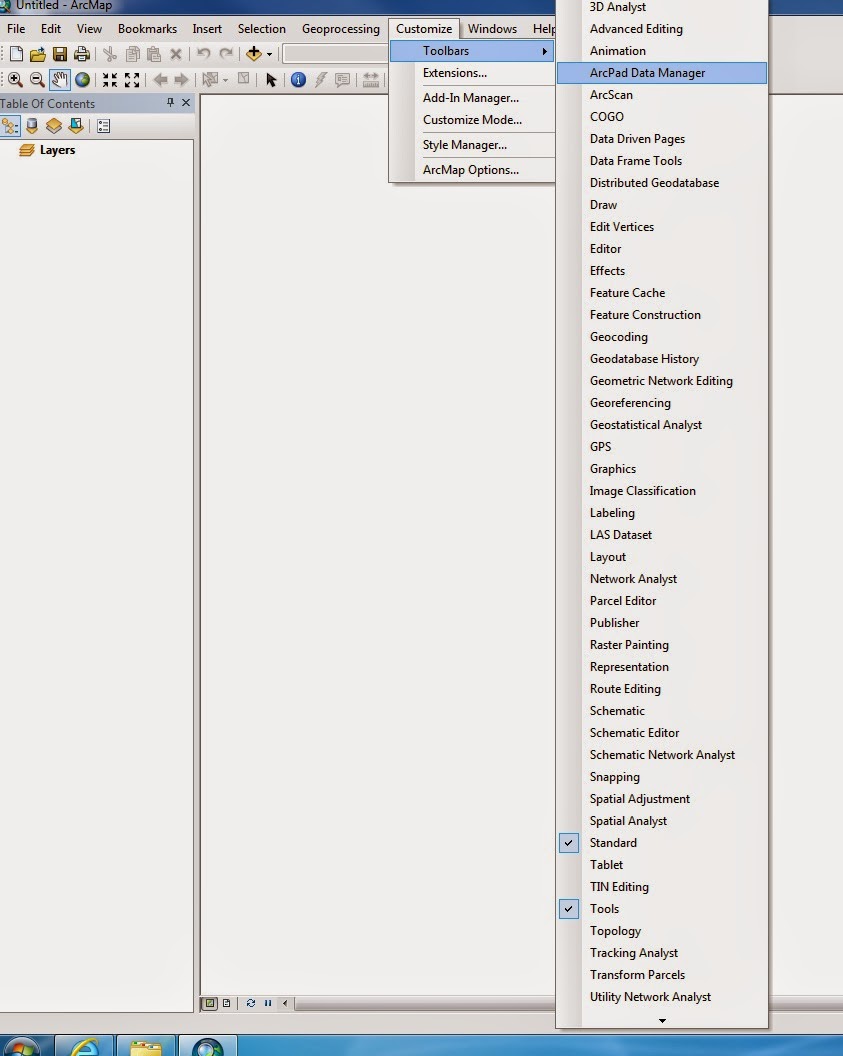
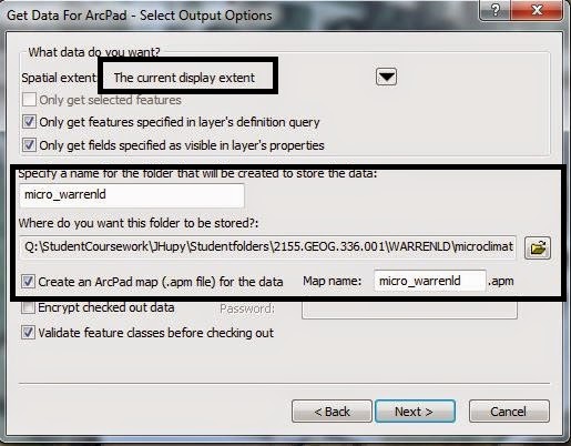
The methods this week were very similar to the previous Exercise (Exercise 6). The objective was to deploy a geodatabase to ArcPad by using ArcMap, collect micro-climate data points from the UWEC campus, then come together and pool the data from each group for a larger scale micro-climate of the campus.

Since the class wanted as much data as possible, the campus was divided into several zones and each group was assigned a zone. The exercise required each group to collect 100 points, but because of time restraints and problems occurring each group collected 50 points.

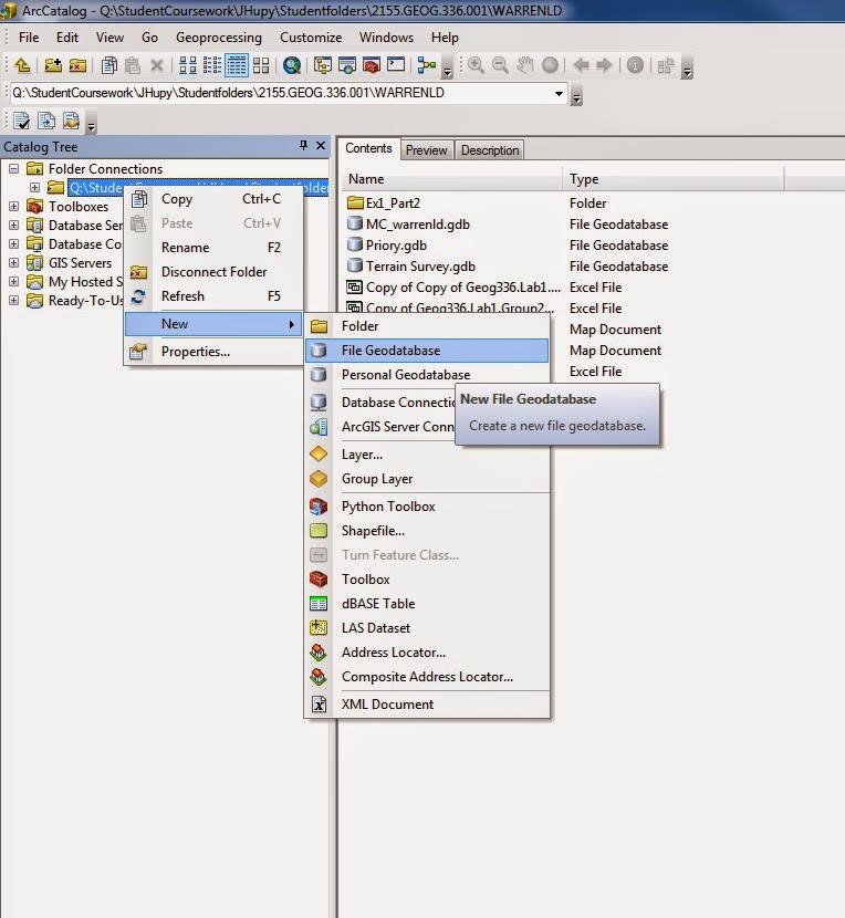
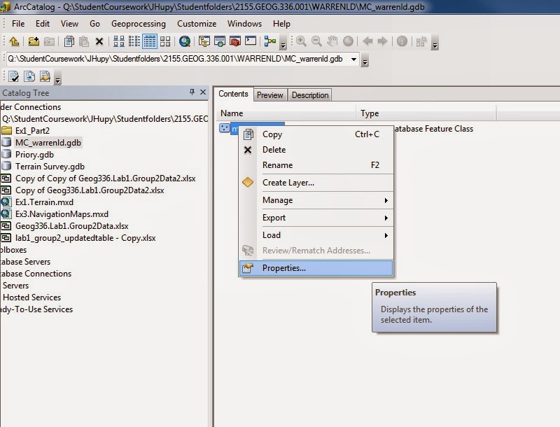
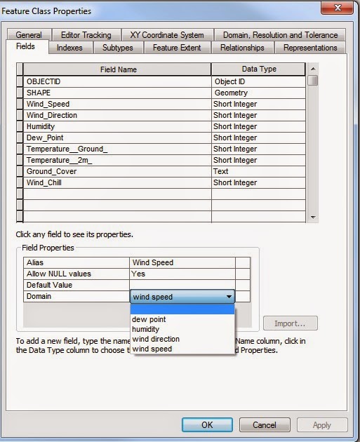
One person from the class developed a geodatabase for all to use after Exercise 6. This was a geodatabase that was very similar to the previous used with fields for microclimate data including wind speed, wind direction, wind chill, temperature, dew point, and humidity. The same domains were developed and used, and a microclimate feature class was formed. This geodatabase was made accessible through it being placed into the class data folder on the Q:\\ Drive. By using the same geodatabase and map project (.mdx), the data would easily be able to be combined into one file and then placed onto the Q:\\ Drive for all to access.

Once the data was retrieved, the IDW raster interpolation method was once again used to display the data. By using IDW, it allows the data points to be formed into a continuous surface map.

Results

 

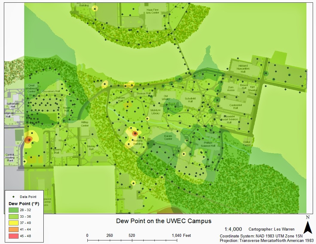
Figure 1. Dew point on the UWEC campus. The map is being displayed as a continuous surface by using the IDW raster interpolation method.  

 

Figure 2. Humidity on the UWEC campus. The map is being displayed as a continuous surface by using the IDW raster interpolation method. Humidity was taken as percent humidity.

 



 

 

Figure 3. Surface temperature on the UWEC campus. The map is being displayed as a continuous surface by using the IDW raster interpolation method. Temperature was taken at the ground level in degrees Fahrenheit.

 



 

Figure 4. Temperature on the UWEC campus. The map is being displayed as a continuous surface by using the IDW raster interpolation method. Temperature was taken at 2m from the ground in degrees Fahrenheit.  

 



 



 

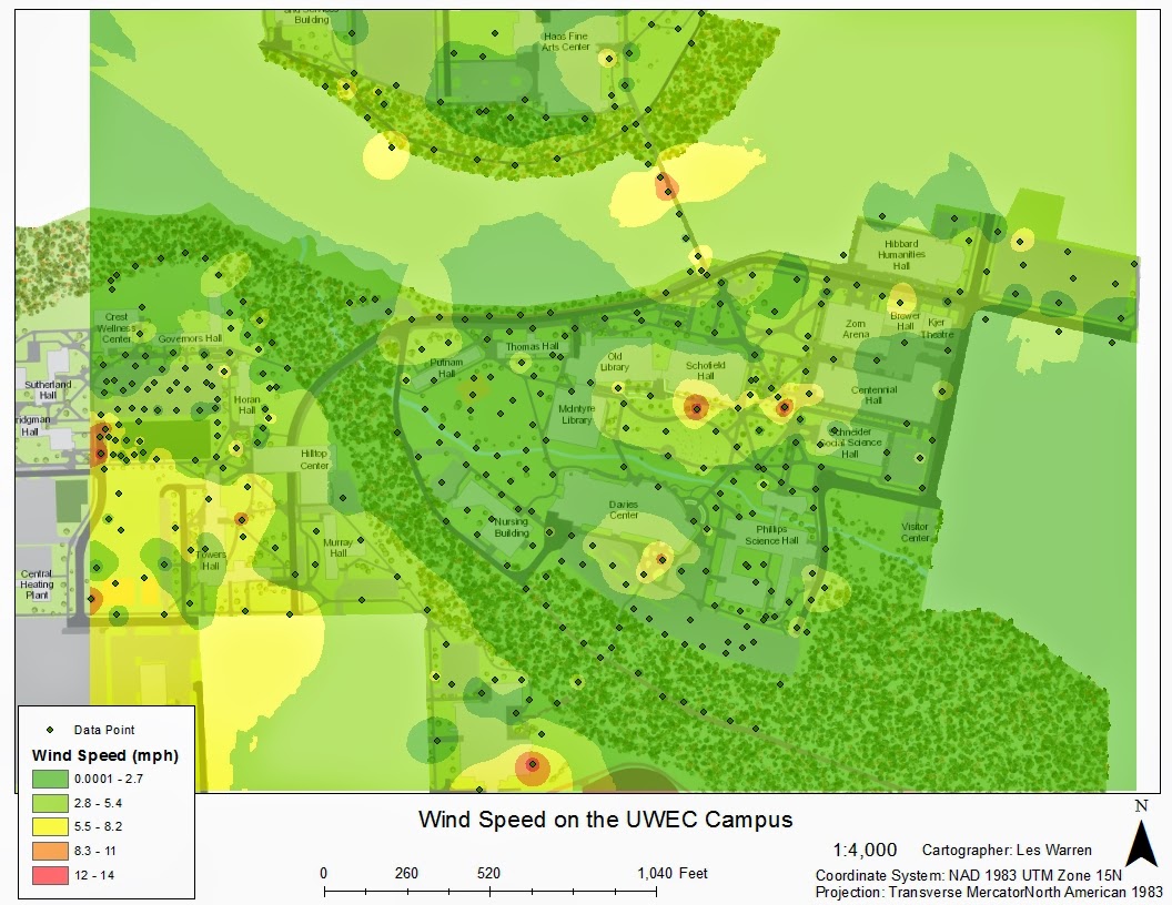
Figure 5. Wind speed on the UWEC campus. The map is being displayed as a continuous surface  by using the IDW raster interpolation method. Wind speed was taken in miles per hour (mph). 

 

 

 

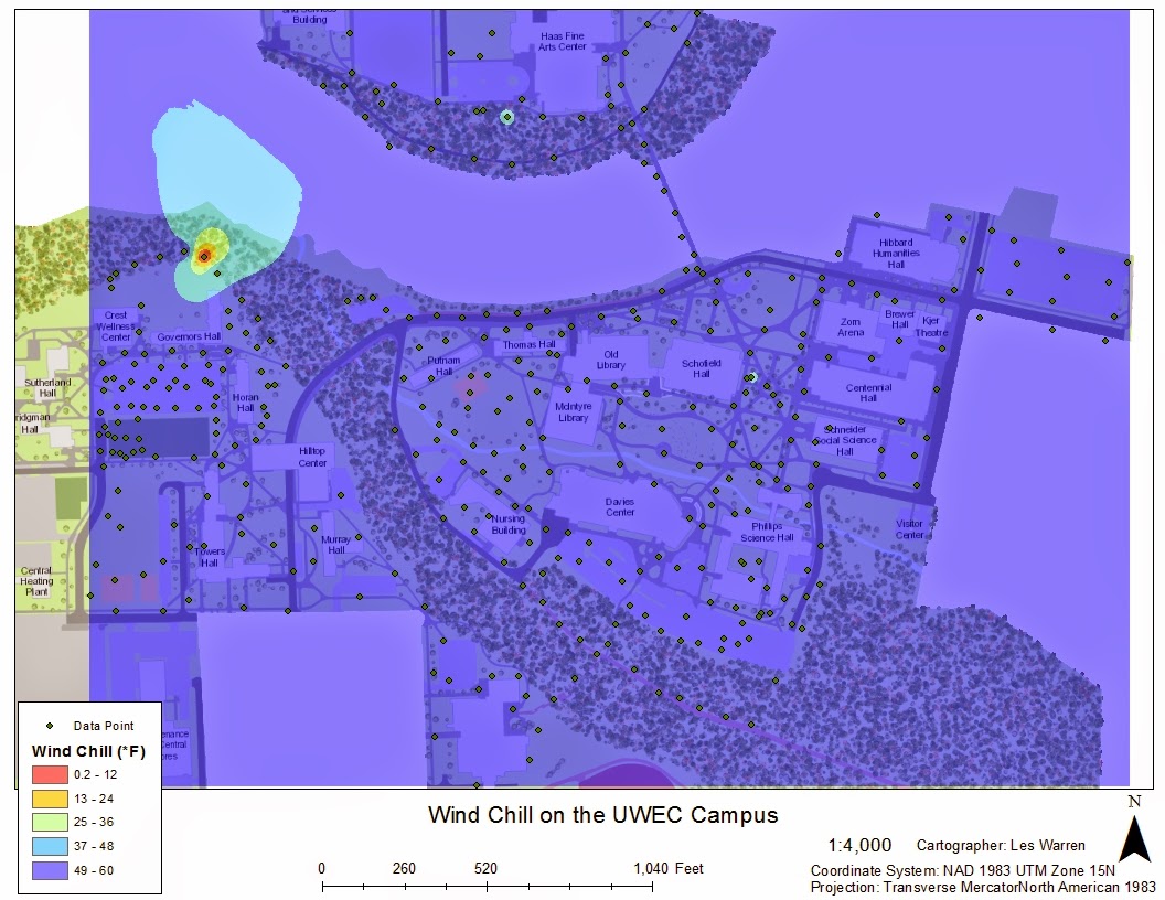
Figure 6. Wind Chill on the UWEC campus. The map is being displayed as a continuous surface by using the IDW raster interpolation method. Wind chill was taken in degrees Fahrenheit.   

Although the campus is a pretty wide spread area of multiple elevations (lower and upper campus) and areas on the river corridor, the microclimate does not vary greatly over the campus. The dew point does not vary at all over the campus, except for distinct spots, but these could have been errors in collection (Fig 1). One of the most varied microclimate variables was the humidity (Fig 2). Neither temperature or surface temperature varied over the campus (Fig 3/4). Both show cooler areas in wooded areas, but if the notes were evaluated, these would most likely be shaded areas. Wind speed also stayed consistent except for some areas of higher elevation and along the river corridor (Fig 5). Finally, the wind chill did not vary at all and was consistent over the entire campus between 49 and 60 degrees.

Discussion/Conclusion

Although this exercise was the same as the previous week except on a much larger scale, implications still occurred. The largest implication was the permissions set on the geodatabase. Although all students could copy and use the geodatabase, we were not able to check data back in or modify the document. This was due to many students just coping and pasting the file it was stored in, rather then the geodatabase itself. One student was able to gain access and checked in all of the ArcPad units into his computer to form the master map project file.

Once again compasses were not supplied or accessible, so wind direction was not measured. Estimates could be made, but not exact values for analyzing or creating a map.

This was the greatest implication since the instructor was not present for this exercise. Although this would not happen for most classes, it was a great experience since we all had to work through the implications and divided the tasks up ourselves. By doing this, we were able to form team work and use knowledge individuals shared to solve problems.

Exercise #6: ArcPad Data Collection and Deployment

Introduction

Easier methods to data collection are up and coming every day in the geospatial world. With the evolvement of the geodatabase, data collection in the field has become easier. The use of handheld GPS units allows researchers to get exact point locations, but also collect data into the geodatabase. With setting up domain ranges, it prevents error in data entry and/or allows you to use coded entries that includes a list of options. The geodatabase also gives the list of data entries needed like ground cover and wind speed. By inputting the values into the GPS, it saves time compared to manual imputation into a spreadsheet or program and directly transfers the data to the feature classes specified.



Study Area

The study area for this exercise consisted of the University of Wisconsin- Eau Claire campus. We were to pick an area of our choosing, but try to get diversity in our environments and not stay within one area. Specifically, my group chose to survey the lower campus the included the surroundings of the academic buildings, campus green space, and the river corridor (Fig 1). The weather observations were cloudy, cool (low 20's), and breezy.

Figure 1. Map of UWEC Lower Campus.

Methods

If recalled in Exercise #5, we were to develop a geodatabase to collect micro-climate data. This week we were to pick up from that exercise and prepare and deploy the geodatabase for collection with ArcPad. To begin, we were to use ArcMap to prepare a map project to deploy and check the data back into. In this project, the first step was to open the feature class that was created last week with the micro-climate fields. The next step was to then add a basemap for a visual while collecting. This was to be our choosing, and our group chose to use the Eau Claire County Ortho Map that was available in the Q:\\ Drive on the school database.



The next step was to deploy the geodatabase to ArcPad to collect data. To do so, the ArcPad Data Package must be activated in the Extensions in the options of ArcMap. Once activated, the ArcPad toolbar can be viewed and used (Fig 2). On the toolbar, the deploy button can be hit, and the tutorial window will pop up (Fig 3). The next button can be hit on the introduction. Next you must hit the "deploy all data and layers" (Fig 4; Fig 5).  Next, you will want to establish a file name and choose the location where the file will be saved (Fig 6). Make sure the Create file on this computer box is checked, and the finish button can be hit (Fig 7). ArcMap will then prepare the file for use on the ArcPad program.

Figure 2. Location to access the ArcPad Toolbar in ArcMap.

 

 

 

Figure 3. ArcPad Toolbar in ArcMap. The button labeled 1a is used to deploy the geodatabase for data collect. Button 1b is used to check in data after data collection.

 

 

 

Figure 4. Deployment tutorial showing how to check out all layers for deployment. To access the menu, the user must right click onto the "Action" bar.

 

 

Figure 5. Tutorial screen showing that all layers have been checked out and the user is ready to move on in the tutorial.

 

 

Figure 6. The third screen of the deployment tutorial. User will want to make sure that the spatial extent is set to the current display extent, choose a file name, choose the location to save the file, and to create a ArcPad map (amp) file and name it.

 

 

 

Figure 7. Last screen of the deployment tutorial. User will want to create the ArcPad data on the computer now and Finish the tutorial for processing.

Within your files, you will now find a file that you named during set-up. Copy and Paste this file into the same folder to have an extra copy of contents incase something goes wrong with the original.

To collect data, a Trimble Juno 3B handheld GPS unit will be used. This unit contained the ArcPad software (Fig 8). To load the files onto the GPS, we plugged the GPS units into the computer and copied the deployment file to the SD card in the GPS. The geodatabase is now ready to collect data.

Figure 8. Example of the handheld Trimble Juno 3B GPS unit used for data collection.



To collect data, a Kestrel handheld weather station was used (Fig 9). This unit was able to tell the wind speed, wind chill, temperature, humidity, and dew point. The only information it could not tell was the wind direction. Along with these variables, the surface type and any notes were also recorded. By using the geodatabase, data collection was easy. By hitting a new data point on ArcPad, it recorded the GPS location and gave input fields for each of the variables. The wind speed, wind chill. temperature, humidity, and dew point were all manual inputs that numbers must be entered. The ground type was a coded domain, so choices were given in a drop down option. The notes category was also a manual typing method.

Figure 9. Example of the Kestrel handheld weather station used for data collection.

Temperature was recorded at both the surface (ground level) and 2 meters up from the ground in degrees Fahrenheit. The wind speed was recorded by placing the unit in the air above the human body in miles per hour. Dew point and humidity were recorded in whole values.



When all data collection was complete, the GPS was then pulled back into the computer. By copying the files off of the SD card and pasting into our personal folders, ArcMap then can check in the data using the check in button on the ArcPad toolbar (Fig 10). The data points should now show up onto the basemap and the attribute table should be full.

Figure 10. Tutorial screen for Checking-In data after collection. The green button in the upper right hand corner allows user to navigate to the folder holding the data. Once data is located, the feature class(es) that need to be checked in can be selected and "Check In" can be hit to finish the process.

After the data has been checked in, raster interpolation methods can be used to form a continuous surface map. In this case, IDW was used to form multiple maps of different microclimate attributes.

Results of Microclimate Survey

  Figure 11. Map of Dew Point on the UWEC Lower Campus. All readings are in degrees Fahrenheit.

 Figure 12. Map of Temperature on the UWEC Lower Campus. Temperature readings were taken at the ground level. All readings are in degrees Fahrenheit.

 

 Figure 13. Map of Humidity on the UWEC Campus. Readings are in percent humidity.

 

 Figure 14. Map of Temperature on the UWEC Lower Campus. Temperature readings were taken at the 2 meter mark above ground. All readings are in degrees Fahrenheit.

 

Figure 15. Map of Wind Speed on the UWEC Lower Campus. Readings are in Miles per Hour (mph).

Overall, the microclimate of the Lower UWEC campus seemed to vary a lot. Higher dew points were found along the river corridor (Fig 11). Temperature at the ground height was found cooler along the river corridor when compared to in-land campus (Fig 12). This was also found for the temperature at the 2m height above ground (Fig 14). The humidity rose as one got closer to the river (Fig 13). The wind speed varied greatly over the lower campus and no distinct pattern was seen (Fig 15).


Discussion

This was a great exercise to learn about ArcPad, the steps to deploy and check in a geodatabase, and some of the implications that can occur. Although we looked at weather, it the was the ideas behind the exercise that were the most valuable.

Although programs like ArcPad make data collection easier, there are many implications that can occur. One issue observed was getting the data to deploy in ArcMap. UWEC has their own campus basemap that could be used to simply show the buildings, parking lots, and other land features. Although it is a basemap, we were not able to get it to deploy for the GPS. After trouble shooting, it was decided it was much easier to use a DEM map that was already on file.

After deployment some data collection errors also occurred. Without a compass, wind direction was not able to be measured. Some other implications I also observed was the way the Kestrel unit needed to be held to record certain variables. It needed to be held higher for wind speed and wind chill, while different temperatures could have been observed it not enough time was given for the unit to adjust.

Although these maps show varied results for the lower campus, only 20 data points were collected. This is a very small amount of data points and to see true differences then more should be collected.


Conclusion

This was a great way to look at what a geodatabase can do besides store data. With techniques like this one, it can simplify the collection and imputation process tremendously. It was also interesting to see how weather patterns can change over a short distance (like a college campus) depending on different ground covers and proximity to bodies of water. Geospatial technology is truly amazing with the applications one can utilize. Although it seems ArcPad is becoming a little outdated, it was still a excellent introduction to mobile data collection.

Exercise #5: Geodatabase

Introduction

The creation of a geodatabase is one of the most important steps when creating and storing data. Geodatabases are the new frontier in geospatial data storage and allow us to easily store data in a neat, organized fashion with files that classify data and contain metadata.

Geodatabases also allow us to set domains ranges to our data. A domain range is the valid values for a particular element in the geodatabase. An example in our case would be temperature. This time of year we know temperature should be between -20 and 60 degrees, so by setting a range on the data it allows us to check for errors while inputting the data. On other field values, we can also set up coded values. These a predetermined values that you can choose from when entering data. These are helpful since it can eliminate typing errors and time while inputting.

Tutorial

The first step in creating a geodatabase is to open up ArcCatalog. In ArcCatalog, you will want to right click on the folder you wish to place the geodatabase in. From there you will want to select "New," then select a "New File Geodatabase" (Fig 1). Depending on the work you are preforming you can choose from either a Personal or File Geodatabase. With a Personal Geodatabase, the space is limited and it must also be stored and accessed in Microsoft Access. It is recommended in most cases to use a File Geodatabase.



Figure 1.

The geodatabase has now been created and can be seen in your designated folder (Fig 2). You will now want to created a new feature class in the designated geodatabase. This can be done by right clicking on the geodatabase and choosing "New" and "Feature Class" (Fig 3). You want to name the Feature Class and choose the type. In this case, we will use a point type feature class. The feature class should now be visible your geodatabase (Fig 4).



Figure 2.

Figure 3.

Figure 4.

The nest step in creating a geodatabase for deployment is the addition of domains. As recalled, a domain range is a set of valid values for the field. A coded domain may also be used to give a lost of choices during data collection. To start adding domains, you will want to right click on your geodatabase in the menu and choose properties (Fig 5). In the tabs on the Database Properties window, you will want to select Domains (Fig 6). To add domains, you will want to name the domain. This will must likely correlate to the data you will be using the domain for. An example for this exercise is wind direction. You can then enter a description of the domain for other users to see in case there are any questions about the domain. In the lower part of the window, there are the domain properties (Fig 6). This allows you to set the minimum and maximum values for the field, the field type (if numeric, text, etc.),  and split and merger policies. For our example of wind direction, we will be measuring the direction from which the wind is coming from with a compass. True North will be 0 degrees. Since we will be using a compass, the minimum value will be 0 and the maximum will be 360 since there are only 360 degrees in a circle.



Figure 5.

Figure 6.

You can add as many domains as needed for the number of fields you have for data collection. Another option is a coded domain. By using a coded domain, a list of options appear for the field when collecting data. For this example, ground type will use a coded domain (Fig 7). By using the coded values option on the bottom, options can be entered like grass, concrete, etc. It is always important to enter a description of the code so that any user can use it for reference if questions occur.

 Figure 7.

 

 The next step is to apply these domains to your fields. By right clicking on the feature class and choosing properties, the Feature Class properties window will appear (Fig 8). In the Feature Class Properties window, you will want to add all of the fields of data you will be collecting (Fig 9). In this case, it includes wind speed, wind direction, humidity, temperature, ground cover, dew point, and wind chill. In the data type, you will want to choose the type of data that will be entered (Fig 10). This includes short integer, long integer and text. You will need to choose the correct type so that when data is entered, it is placed into the correct format (like how many decimal places to include).

 Figure 8.

 

 Figure 9.

Figure 10.

For each field, you will also be able to select the appropriate Field Properties (Fig 11). The Alias will show up as the name of the field as you specified above. You have the option to except null values if wished, and also specific a domain. When you click to specify a domain, a drop down lost will appear with all of the domains you added earlier (Fig 12). Choose the appropriate domain for each field type.

 

Figure 11.

Figure 12.

Now that all fields and domains have been applied, you are now ready to deploy the geodatabase and collect data!