Exercise #4: UAS Background

Introduction

Unmanned Aerial Systems (UAS) are the up and coming future of geospatial technology. An UAS is a  remotely controlled aerial vehicle. They can be used for a variety uses including remote sensing, aerial surveillance,  and land surveying. With the ability to carry multiple kinds of cameras and sensors, the number of uses is countless and continues to grow. Types of sensors include biological, chemical, and electromagnetic spectrum sensors. These sensors can take aerial imagery, monitor air control, and even detect microorganisms.

In this lab, we were to spend two hours on RealFlight 7.5. RealFlight is a simulator program for UAS aircraft. These aircraft range from the most simple to the most complex systems. It also allows you to change environmental factors like weather and different locations and scenarios to fly. The second part was to then research the uses of different aircrafts and sensors, and then respond to given scenarios.

Flight Simulator

During the use of the RealFlight 7.5 simulator, we were to use four different aircraft over the two hour period (approximately a half hour on each). During this flight time, we were not only to learn to fly the aircraft, but also change environmental factors to challenge ourselves.

Over the two hours of simulation time, I flew four different aircraft that included a Slinger, Quadcopter, Octocopter, and a Mitsubishi Plane. Starting with the most basic, the Slinger was a good way to get used to the controls and different camera views. A Slinger is one of the cheapest and most basic of UAS aircraft (Fig 1). They are most commonly made of a Styrofoam material and come in a variety of shapes and sizes. One of the most difficult things to learn about the Slinger was proper take off technique and keeping it level while flying.

Figure 1. Example of the Slinger aircraft used during simulation.

 



 A Quadcopter is the next step up in UAS aircraft (Fig 2). Driven by four propellers, this aircraft is easily flyable and can hold more weight then more basic models. The Quadcopter is easily flyable on take off, but is more difficult to keep steady and on a straight path in the air. It is also easily landed with the downward arms as support.

 



Figure 2. Example of the Quadcopter aircraft used during simulation.

 

 The Octocopter is very similar to the Quadcopter with being a multi-rotor aircraft, but has eight propellers for maximum lifting power (Fig 3). Although a aircraft like this can lift more weight, it also has a downfall of less battery life with more propellers to run. This aircraft seemed to be more steady in the air then the Quadcopter.

Figure 3. Example of the Octocopter aircraft used during simulation.

 



The last aircraft used during simulation was a Mitsubishi plane. I choose this aircraft to see the differences in the Slinger vs. a plane model. I found aircraft like these were more easy to fly then the multi-rotor since you could fly a straight path. I would say aircraft like these are better for larger areas, whereas multi-rotor would be better suited for smaller areas.

Figure 4. Example of the Mitsubishi plane aircraft used during simulation.

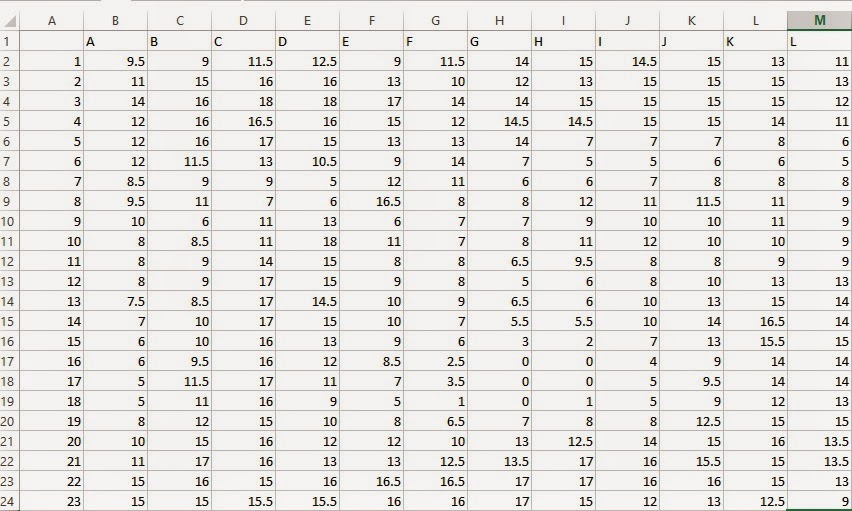
All flight conditions and results were logged (Fig 5). This is a good way to record flight time along with any difficulties and reasons for future missions. Unmanned Aerial Systems can save companies and departments money, but also can cost if not properly used or the pilot has minimal experience.

Figure 5. Flight log of simulator aircraft, time, conditions, and result of flight.

Scenarios


1) An oil pipeline running through the Niger River delta is showing some signs of leaking. This is impacting both agriculture and loss of revenue to the company.

A multi-rotor UAS is going to be most effective at maneuvering around the Niger River delta. The multi-rotor UAS has ability to move in all directions and will allow for the most land to be covered in a short period of time. One of the draw backs to using the rotary UAS is that it has a very short battery life. Some potential sensors would include a UV Sensor to detect the oil and vegetation or a Near-IR (NIR) would also be able to do the same.

2) A military testing range is having problems engaging in conducting its training exercises due to the presence of desert tortoises. They currently spend millions of dollars doing ground based surveys to find their burrows. They want to know if you, as the geographer can find a better solution with UAS.

An option that would be effective at solving the desert tortoise problem in the most effective and inexpensive way would be to use a Slinger (fixed wing) UAS. The Slinger would be the best UAS for this particular job because it has the longest flight time and range. It is best for aerial mapping and making terrain modeling of large area. An UAS that is able to cover large distances will be best for this job. Some possible sensors would include a TIR or TAR, since they are best at looking at surface temperatures, which are important with Tortoises.

Exercise 3: Navigation Maps

Introduction

 

In the third exercise for class, we were to create navigation maps that will be used in a later activity in the semester. The area to be mapped, the Priory in Eau Claire, WI, will be the location of several navigation course points that must be manually mapped and navigated using compasses and pace counts. The data for the exercise was provided to us by Dr. Joe Hupy and located in the Priory geodatabase on the Geography Department Q:\\ Drive.

 

Methods

 

 

To complete this exercise, majority of the data was provided, but we were required to use both cartography and GIS skills learned and used in previous coursework. To start, the data provided in the geodatabase was reviewed and explored to look at the provided data and to start thinking about what data needed to be used.

 

It was totally up to each individual person to construct his or her map and which data to include. Something to always keep in mind is the use of the map and to not over do the map with including too much data that the map is not easily readable. Some options provided were 2ft contour lines, 5m contour lines, no shooting zones, navigation boundaries, point boundaries. and areal photography of the area. This data was provided to save time on our part, and to also focus our efforts onto the map making process. The data was obtained from the USGS and previous UW-Eau Claire studies of the area.

 

 

Some requirements were provided to us in the mapping process. We were to include a north arrow, scale bar, reference scale, information on the coordinate system and projection, a properly labeled grid, list of data sources, and our name. We were to also choose a suitable background of our choice from either the Priory geodatabase or the base map options on ArcMap.

 

 

The first step in the cartography process was to establish the area to be mapped. To begin, the navigation boundary was loaded into ArcMap. To make the area transparent, a hollow fill and black border were selected for the rectangle. Next, the suitable background was chosen. After exploring several options including aerial imagery from online and the aerial photos from the geodatabase, the aerial photos from the geodatabase seemed to work the best. We were also to select a given coordinate system and UTM was chosen. This was to help reduce distortion in the given area and also provided easily measurable units that could be used in navigation. All of the features were projected into the NAD 1983 UTM Zone 15 coordinate system with a Transverse Mercator projection.

 

 

Now that the area of study had been established, it was time to begin adding data that would be suitable for navigating the area. For my maps, I chose the 5m contour lines over the 2ft contour lines because the  5m lines were much clearer and easier to read, but also worked well with the scale of the map, which was set in meters. The point boundaries were also placed onto the map to help contain the selected area of the points during navigation.

 

The last steps were to create two cartographic pleasing maps in ArcMap. One map was to include a UTM grid at 50 meter spacing (Fig 1), while a second map was to include a grid in decimal degrees(Fig 2). The grids were placed onto the map by using the grid options under the layer properties. The grid options allows you to select the type of grid (gratitude or measured grid) and also provides the labeling and font options. Within the layout view on ArcMap, you can easily format, add, and position objects onto your map. This is where the scales, legend, titles, and text can be added along with adjusting the size and view of your dataset.   

 

The map can then be exported into the selected format of your choice, in this case, PDF.

 

 

Figure 1. Map of Priory with UTM grid set at 50 meter spacing.  

 

Figure 2. Map of Priory with Decimal Degree Grid set at a 5 degree spacing.

Discussion

In the navigation of the selected course points in the upcoming exercise, these maps should be very useful. The contour lines provide information on the sloping on the terrain, and having the boundaries of the Priory will provide information if you are off track. Lastly, the aerial imagery will be useful in the identification of terrain areas (grass, forest, etc.) and landmarks.

As with all maps, some problems and implications could arise. Much of this data was taken some time ago, so certain terrain types or landmarks may have changed. Also, the contour lines do not include values as to if the terrain is sloping upward or downward.

Conclusion

This exercise was a great way to review previously learned cartographic techniques and also the thought processes behind data selection. Every map has a purpose, and a lot of thought should go into the data needed so that the map is not overly done, but also includes enough data for the job. These maps should be useful in the upcoming exercise to successfully navigate and measure.   

Exercise 2: Visualizing and Refining Terrain Survey

Introduction


In the second part of the terrain survey exercise, we were asked to conduct three different steps to complete the analysis of the terrain that the group formed in part 1. First was the importation of the X, Y, Z coordinates and creating a feature class. Next, 3-D analysis tools were used to visualize the terrain in various ways. Lastly, the group was able to resurvey areas of the terrain to help improve weak areas on the visualization and choose the best analysis tool for the given terrain. To visualize and analyze the terrain, we used the following tools in ArcMap:

• IDW
• Kringing
• Spline
• TIN
• Natural Neighbors

Methods

The second part of this lab exercise started with us preparing our spreadsheet into a format that could be easily imported into ArcGIS and be created into a feature class. The spreadsheet was put into an Z,Y,Z format and then formed into a new feature class in ArcCatalog. The feature class formatted the 276 data points into a formation similar to the grid used on the sandbox during the survey (Fig 1).

Figure 1. Point formation formed by ArcMap after the importation of the X, Y, and Z values to a new feature class. This formation is similar to the grid used for the survey.

 

 

The next step was to use the 3-D analysis tools in the ArcMap toolbox to begin the visualization process. The raster interpolation tools were used to visualize the date. Interpolation is the method of  estimating surface values at unsampled points based on known surface values of surrounding points The tools used included IDW, kringing, natural neighbors, spline, and TIN. Once the 3-D tool had been preformed on the feature class, then the data was saved to a layer and opened up in ArcScene. ArcScene takes the layer information and projects the data into a 3-D version.

 

 

IDW is a 3-D analysis tool that interpolates a raster surface from points using an inverse distance weighed technique. This technique has its disadvantages because it is limited on the range of values used and is weak when the highest or lowest extremes have not been already sampled. But it has advantages when the sample points are dense, but is limited to a maximum of 45 million input points. Figure 2 shows the IDW method in ArcSecne.  

Figure 2. 3-D view of the IDW interpolation method in ArcScene of the terrain surveyed.  

 

 

Kringing is the interpolation method that uses a processor-intensive process. This may be a down fall becasuse the time of processing depends on the number of points and size of the search window. One advantage is that an optional output of prediction variable can be calculated to evaluate the need for more data points. Figure 3 shows the terrain using the kringing method showed in ArcScene.

Figure 3. 3-D view of the kringing interpolation method in ArcScene of the terrain surveyed.

 

Natural neighbors is the interpolation method that imploys the use of a natural neighbor technique. Disadvantages of this technique is that it has a limit of 15 million data points, and it is reccomended to study the area in sections rather than one large area. It is also recommended that the data be in a projected coordinate system than a geographic coordinate system. Figure 4 views the natural neighbor method in ArcScene.



 

 

Figure 4. 3-D view of the natural neighbor interpolation method in ArcScene of the terrain surveyed.

 

Spline is the method that interpolates a raster surface using a 2-D minimum curvature spline technique. A advantage of this method is that the smooth surface passes exactly through the impout points and with a larger number of points, a smoother surface can be formed. Figure 5 shows the spline method in ArcScene. We determined this to be the best method for our surveyed terrain sample.  

 

Figure 5. 3-D view of the spline interpolation technique method in ArcScene of the terrain surveyed.

 

 

A TIN creates an image using a triangular irregular network. The tool used was Create a TIN in the 3-D analysis tools and must be used with a projected coordinate system. It is also recoomended to limit data points for display performace. Figure 6 shows the 3-D TIN in ArcScene. 

 

Figure 6. 3-D view of the TIN interpolation method in ArcScene of the terrain surveyed.

 

 

After all interpolation methods were performed, the group analyized each one to decide on the one with the best fit for our surveyed terrain. As mentioned above, the group decided that the spline method was the best fit due to the smooth visualiztion fitting our hills and ridges well. There was one area that was seen on all of the 3-D visuals that did not fit the terrain well. The valley/ridge was shown as a tall point on the map, rather than a long, narrow spot. The group resurveyed the terrain in the 60 x 50 cm area, and to increase the visualization, twice as many points were collected in 5cm intervals, rather than the original 10cm intervals and inputed for that area. The new grid is shown in figure 7.

 

 

Figure 7.  Point formation formed by ArcMap after the importation of the X, Y, and Z values. The condensed area of points is the area that was re-surveyed after the inital visualizations.

 

After the new X, Y, and Z points were inputed and a new feature class was processed, the spline method was used again and viewed in ArcScene (Fig 8).  

 

 

Figure 8. Refine of spline method after additional data points were collected. The image is viewed in ArcScene.

Discussion


The 3-D visualizations seemed to be pretty accurate for the terrain that we created and surveyed. It is definitely accurate to say that a symmetrical grid is always needed. Areas with large terrain shape change, like a hill or valley need more input points, while flat areas need less. Also, the more points collected, the more accurate overall. Although I think we did a pretty good job on the number of points collected in most areas, but some areas of large terrain change could still probably use some resampling to obtain more data points.

Some implications of the exercise could include the measuring of our grid system since precise instruments were not used, but also the values in the spreadsheet. It is very easy for a person to type a wrong value in or miss hit a key on the computer. A large implication of the resampling process is that the resample was done one week after the original survey. Snow was used to build the terrain, so depending on the weather, the terrain could have changed in height over the week.   



Conclusions


This was a great exercise overall. It was definitely interesting to be able to use and see how the software works from our own creation. Although all visualizations worked well, some worked better then others. The spline was best for our terrain, but I think the largest question is looking at the type of data you are using and how many points were collected.

Exercise 1: Survey of Terrain Surface

Introduction

The first field activity that we performed in the class was taking a survey of the terrain of an area that the group designed. This activity was designed to engage in geospatial thinking and develop critical thinking skills. Working in a the field of geospatial technology definitely takes critical thinking skills no matter if you are developing a new computer program, making a map, or collecting field data.


Methods

The exercise was performed in the courtyard of Phillips Hall on the University of Wisconsin Eau-Claire campus. Each group was assigned a garden box to build terrain and develop a survey technique to use. Within the garden box, the group could use any material to build a terrain, which in our case, snow was used to form a landscape. The terrain varied from ridges, valleys, plains, depressions, and hills (Fig 1).

On Wednesday, January 28, 2015, the group met up to build and survey the terrain. Weather conditions consisted of  mid- 20 degree weather and cloudy. The wooden edges of the garden box marked sea level and the box measured out to be ~ 112cm x 240 cm.

Figure 1. Top view of the terrain surface developed from snow in the garden box.

 

 

The terrain was surveyed using a X/Y plot method. Both the X and Y axes were measured out into 10 cm increments (Fig 2). String was then used to form a grid so that measurements could be easily taken. The string grid marked where the measurements on the X/Y axes should be taken, but also was the marking point of sea level. The yardstick could then easily be used to measure the Z (depth) value from the terrain to the string marking sea level (Fig 3). The measurements were recorded into a field notebook and then transferred into excel (Fig 4). The X axis was labeled A- L and the Y axis 1-13. All Z values were negative due to all terrain being below sea level. 

 

 Figure 2. Top view showing the grid layout. String and tacks were used to mark 10 cm increments on both the X and Y axes for a total of 276 measurements. Terrain height was measured in cm from terrain up to the string marking sea level.  

 

 

Figure 3. Students measuring terrain using a yard stick and recording values in a field notebook.

Figure 4. Excel file showing measurements.

Discussion

The use of the grid method made the taking a the terrain measurements easy and quickly. With laying the grid out into 10cm x 10cm increments, all of the different terrain was able to receive multiple measurements and the entire garden box was surveyed. With the use of the yardstick to both layout the grid and take measurements, accuracy was one variable that could be an issue. Ample time was taken to lay out the tacks and string to ensure accuracy, but some variance should be expected. Also with multiple students from the group taking measurements, it also becomes another variable on accuracy.


Conclusion

Overall, this exercise tested the minds of the students and developed critical thinking skills. Myself and other students were made to think hard on the techniques used and the situation at hand. Many different techniques could have been used, but thinking critically on each one helped develop skills for different situations in the future.